The MANOVA Test
Extend ANOVA test capabilities using multivariate analysis of variance

Complete the form below to unlock access to ALL audio articles.
Multivariate analysis of variance (MANOVA) is an extension of the commonly used analysis of variance (ANOVA) method, allowing statistical comparisons across three or more groups of data and involving multiple outcome variables at the same time. This article will cover the theory underpinning MANOVA, the types of MANOVA and a worked example of the test.
What is MANOVA?
Multivariate ANOVA formula
MANOVA assumptions
Types of multivariate analysis of variance
Canonical correlation analysis (CCA) and other multivariate techniques
MANOVA vs ANOVA
When to use MANOVA analysis
MANOVA example and interpretation
What is MANOVA?
MANOVA is a statistical test that extends the scope of the more commonly used ANOVA, that allows differences between three or more independent groups of explanatory (independent or predictor) variables across multiple outcome (dependent or response) variables to be tested simultaneously. It is used when the explanatory variables are categorical (arranged into a limited number of values, e.g. gender, blood type) and the outcome variables are quantitative or continuous (able to take any number in a range of values, e.g. age, height). An example might be that we are interested in the effect of three different medications (explanatory variable) on both weight change and cholesterol levels (outcome variables). MANOVA does this by assessing the combined effect of the groups on the outcome variables based on the means in each of the independent groups.
Multivariate ANOVA formula
MANOVA follows similar analytical steps to the ANOVA method. It involves comparing the means of the outcome variables across each group and quantifying the within- and between-group variance. Some key steps in the calculation are the degrees of freedom (df) of the explanatory variable (the degrees to which the values of an analysis can vary), sum of squares (which summarizes the total variation between the group means and overall mean), the mean of the sum of squares (calculated by dividing the sum of squares by the degrees of freedom).
A step in MANOVA that differs from ANOVA is calculation of the test statistic. There are various test statistics that can be used in MANOVA, each suitable for different situations with regards to overall sample size, group size in the explanatory variable and the assumptions of the test being violated. These include Wilks’ Lambda, Pillai’s trace, Hotelling’s trace and Roy’s largest root. Wilks’ Lambda is most commonly used and so will be the focus of this article.
The formula for the Wilks’ Lambda test statistic in MANOVA is:

Where E is the within-group covariance matrix, which measures variability of the outcome variables within each group of the explanatory variable. A matrix is a set of numbers arranged into rows and columns, and they are commonly used in statistics. T is the total covariance matrix, which includes E plus the between-group covariance matrix (H) which measures the variability of the outcome variables between each group of the explanatory variable. Wilks’ Lambda can then be converted to an F statistic to conduct a hypothesis test.
MANOVA assumptions
Some key assumptions of MANOVA are as follows:
- Multivariate normality: that the outcome variables follow a multivariate Normal distribution within each group of the explanatory variable.
- Homogeneity of covariance matrices: that the covariance matrices of the outcome variables should be equal across each group of the explanatory variable.
- Independence: that the observations in the data should be independent from one another and collected as a random sample of a population.
Types of multivariate analysis of variance
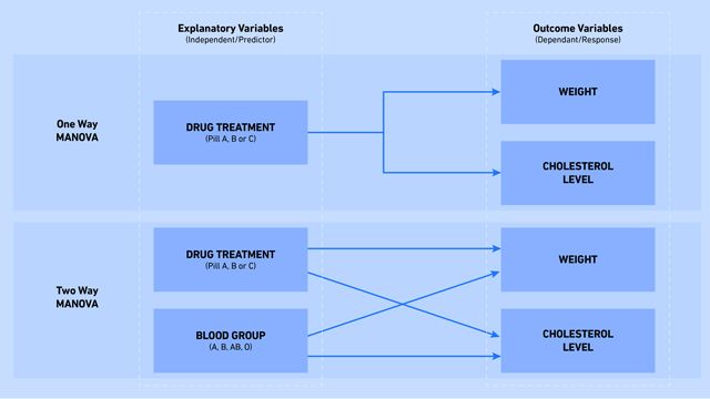
As with ANOVA, even more complex variations of the MANOVA method can be undertaken (Figure 1):
- One way MANOVA: is the simplest form, comparing the means of three or more groups of data.
- Two way MANOVA: extends the method allowing for comparison between three or more groups of data across two explanatory (or independent) variables.
- Repeated measures MANOVA: extends the method to allow the same individuals to have multiple measures across different time points, meaning the data points are not independent.

Figure 1: Differences in comparisons made by one way and two way MANOVA with examples of variables that may be analyzed. Credit: Technology Networks.
Even more complex types of the test can be conducted, including multi-way MANOVA (more than two explanatory variables), and two way repeated measures MANOVA with an additional covariate. Multivariate analysis of covariance (MANCOVA) is an extension to MANOVA where two or more explanatory variables are compared simultaneously.
Canonical correlation analysis (CCA) and other multivariate techniques
MANOVA is one of a group of techniques called multivariate statistical methods. “Multivariate” refers to multiple outcome variables assessed at once, this contrasts with “multiple” or “multivariable,” which usually refers to multiple explanatory variables. Other key techniques include canonical correlation analysis (CCA), where the relationship between two sets of variables is explored by finding linear combinations of the variables that are maximally correlated with each other. Another is principal component analysis (PCA), which transforms a dataset to reduce its complexity while minimizing information loss. Others include cluster analysis, multivariate regression and multidimensional scaling (MDS).
MANOVA vs ANOVA
Let’s consider how ANOVA and MANOVA differ from one another (Table 1).
Table 1: Summary of some key differences between ANOVA and MANOVA.
| Element | ANOVA | MANOVA |
| Covariates | Tests multiple groups of explanatory variable and one outcome variable | Tests multiple groups of explanatory variable and two or more outcome variables |
| Assumptions | Assumptions of normality, independence and variance homogeneity | Assumptions of multivariate normality (for both outcome variables), independence and variance homogeneity (for both outcome variables) |
| Test method | Uses means to calculate variance within and between groups, and an F statistic | As in ANOVA, but calculations done within matrices to deal with the two outcome variables, and an additional step such as Wilks’ Lambda to calculate F statistic |
When to use MANOVA analysis
The main distinction between MANOVA and ANOVA is that MANOVA deals with two outcome variables simultaneously. In some contexts, it would be sufficient to conduct two separate ANOVA tests for each of two outcomes. However, in certain circumstances, such as when the two outcome variables are related in some way, MANOVA allows for a more nuanced analysis by examining them in relation to the explanatory variable simultaneously. In the same way ANOVA is the correct alternative to multiple t tests, MANOVA is the correct alternative to multiple univariate (one outcome variable) ANOVA tests.
MANOVA example and interpretation
Let us take the example of an investigation into the effects of three different medications (explanatory variable) on weight change in kg and cholesterol levels in mg/dL (outcome variables). A one-way MANOVA is appropriate.
Step one: is to calculate the vectors (where a set of numbers is represented together and arranged in a specific order) for each of the three explanatory groups.
If in our investigation we have an overall sample of 200 individuals (full data not shown), let us assume we calculate the following (where the mean weight change for treatment A is 2.3 and the mean cholesterol level for treatment A is 165.4):
Means for treatment A: [2.3, 165.4]
Means for treatment B: [5.5, 200.2]
Means for treatment C: [4.2, 180.8]
Overall mean vector = [(2.3 + 5.5 + 4.2/3), (165.4 + 200.2 + 180.8/3)]
= [4.0, 182.1]
Step two: is to compute the within- and between-group covariance matrices.
The means can be calculated by hand, but due to the complexity brought about by the multiple outcome variables and matrix algebra, this step is only feasible using a statistical software such as Stata or SPSS.
For illustrative purposes, let us assume our within-group covariance matrix (E) is:

In the above, each value in the matrix represents the variability for the outcome variables within the groups. 3.2 is the sum of squares for the weight change variable (variability of weight change values within each group), Both -7 values represent the sum of cross-products between weight change and cholesterol levels (the covariance between the two outcome variables within each group). 35 is the sum of squares for the cholesterol level variable (variability of values within each group).
And the between-group covariance matrix (H) is:

Similarly, each value in this matrix represents the variability for the outcome variables between the groups. 22 and 172 are the sum of squares between groups for the weight change and cholesterol levels respectively. Both 52 values are the sum of cross-products between the outcome variables.
Step three: is to calculate Wilks’ Lambda.
A reminder of the full formula is:

To substitute in the components, we need to use the covariance matrices and the total covariance matrix T to calculate the determinant (the singular value that can be calculated from a matrix) of each line of the formula:

![]()
![]()
![]()
Step four: conduct a hypothesis test.
Next, we can use statistical software to convert the Wilks’ Lambda value to an F statistic and conduct a hypothesis test. The null and alternative hypotheses are as follows:
- Null hypothesis H0: the mean vectors of weight gain and cholesterol levels are equal across all three treatments.
- Alternative hypothesis H1: at least one of the three treatment groups has a different mean vector of weight gain and cholesterol levels.
Finally, the F statistic can be used to derive a p-value (a probability of obtaining an F statistic as extreme or more extreme than the observed results under the null hypothesis), using the degrees of freedom in the analysis and an F-distribution (a probability distribution used in these types of statistical tests). This can be done using F-distribution look-up tables or more commonly by using a statistical software. In our example, the F statistic was found to have a corresponding p-value of p < 0.001. This means we have strong evidence against the null hypothesis of all mean vectors being equal across the treatments. It is important to note that, if these two outcome variables were to be analyzed separately in two ANOVA tests, the results from the hypothesis tests may not have reached the same conclusion due to the interplay between weight change and cholesterol levels with respect to the explanatory variables.
Further reading:
- Penn State University. Lesson 8: Multivariate analysis of variance (MANOVA). https://online.stat.psu.edu/stat505/book/export/html/762. Penn State University. Accessed Jan 17, 2025.
- Gaddis ML. Statistical methodology: IV. Analysis of variance, analysis of covariance, and multivariate analysis of variance. Acad Emerg Med. 1998. 5;3. doi:10.1111/j.1553-2712.1998.tb02624.x
- Bland M. An Introduction to Medical Statistics (4th ed.). Oxford. Oxford University Press; 2015. ISBN:9780199589920
- Frost J. Multivariate ANOVA (MANOVA) benefits and when to use it. Statistics by Jim. https://statisticsbyjim.com/anova/multivariate-anova-manova-benefits-use/ Accessed Jan 28, 2025.


