X-Ray Fluorescence (XRF): Theory, Practice and Applications
X-ray fluorescence is a non-destructive analytical technique used to determine a material's elemental composition.
Complete the form below to unlock access to ALL audio articles.
Since its commercialization in the 1950s, X-ray fluorescence (XRF) spectrometry has become the dominant elemental technique of choice for determining low parts-per-million (ppm) to percentage concentration levels in solid samples, including metals, alloys, ores, rocks, soils, glasses, powders, plastics, paints, ceramics, consumer products, electronics, foodstuffs, plant materials and pharmaceuticals.1
What is X-ray fluorescence (XRF)?
Key components of an XRF spectrometer
Energy-dispersive X-ray fluorescence (EDXRF)
- Handheld XRF spectrometers
- Micro (µ) XRF
- Scanning electron microscopy EDXRF (SEM/EDS)
- Total reflection XRF (TXRF)
Wavelength-dispersive X-ray fluorescence (WDXRF)
EDXRF vs WDXRF: Choosing the right technology
What is X-ray fluorescence (XRF)?
The fundamental principles of XRF spectrometry are well documented.2 A sample is irradiated with a beam of high-energy X-ray photons from an X-ray tube. As the excited electrons in the atom fall back to a ground state, they emit X-rays characteristic of the elements present in the sample. This process is shown simplistically in Figure 1.

Figure 1: Principles of XRF. Credit: Technology Networks.
The individual X-ray wavelengths are separated and measured via a system of crystals, optics and detectors. Elemental concentrations in unknown samples are quantified by comparing the X-ray intensities against known calibration standards. The primary benefit of XRF over other solid sampling techniques, such as arc or spark emission, is that it can analyze both conducting and non-conducting materials as well as inorganic and organic matrices with minimal sample preparation.3, 4
The analytical domain of XRF covers most elements in the periodic table, from magnesium {atomic number (Z) – 12} up to uranium {atomic number (Z) – 92}. However, because the lighter elements below magnesium have much lower energy, very few X-rays are emitted from the sample surface without being absorbed and, as a result, struggle to be detected.
Key components of an XRF spectrometer
There are many different commercial designs of the XRF technique, but it is commonly available in two separate configurations: energy-dispersive (EDXRF) and wavelength-dispersive (WDXRF).
Energy-dispersive X-ray fluorescence (EDXRF)
In the EDXRF approach, the intensity of the photon energy of the individual X-rays is detected and measured simultaneously using multi-channel data electronics controlled by a computer, as shown in Figure 2.

Figure 2: Simplified schematic of an EDXRF system. Credit: Technology Networks.
Some of the many different types of EDXRF technologies available include:
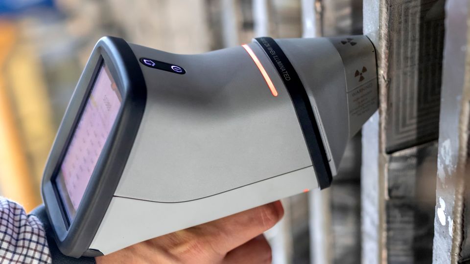
Handheld XRF spectrometers
Handheld XRF analyzers are portable EDXRF devices that can be used in the field for immediate, lab-quality results to help determine the next course of action and where it might be needed.5
The ability to take the XRF technique to remote locations enables the analysis of samples that are too large, unwieldy or costly to transport to the lab. It is mainly used for applications where there is a need to identify a sample’s material chemistry or alloy grade in remote locations and get a result very quickly. It has been applied to a broad and diverse range of industrial materials such as metal alloys, cement, coal, geological samples such as soils and rocks, as well as household materials such as jewelry, paint, electronics and consumer goods.
Micro (µ) XRF
Significant advances in X-ray optics and detectors have facilitated the commercialization of laboratory µXRF spectrometers.6 These instruments offer spot sizes in the ~3–30µm range, enabling routine imaging of element localization within samples.
This type of non-destructive high-resolution elemental mapping could previously only be achieved on relatively small areas using scanning electron microscopy with energy dispersive spectroscopy (SEM-EDS) or by using µXRF beamlines at synchrotron (cyclical particle accelerator) facilities. The development of laboratory scale µXRF spectrometers allows for application across various research and industrial settings. The capability to collect data on element distribution from large and hydrated samples such as intact plants – with performance approaching that of synchrotron beamlines – opens a variety of new µXRF applications in food and agricultural sciences.
Scanning electron microscopy EDXRF (SEM/EDS)
SEM-EDS integrates two techniques: scanning electron microscopy (SEM) and energy-dispersive X-ray spectroscopy (EDS).7 SEM provides high-resolution images of the material's surface by scanning it with a focused electron beam. The interactions between the electrons and the atoms in the sample generate multiple signals, including secondary electrons, backscattered electrons and characteristic X-rays. EDS analyzes the X-ray signals, enabling the determination of the sample's elemental composition. The combination of SEM and EDS furnishes a comprehensive understanding of the materials’ surface topography and elemental composition.
Total reflection XRF (TXRF)
TXRF is a surface elemental analysis technique often used for the ultra-trace analysis of particles, residues and impurities, predominantly on smooth surfaces.8 TXRF is essentially an energy-dispersive XRF technique arranged in a special geometry. An incident beam impinges upon a polished flat sample carrier at angles below the critical angle of external total reflection for X-rays, resulting in the reflection of most of the excitation beam photons at this surface. The sample, deposited in the sample carrier is seen as a very thin sample under a very small angle. Due to this configuration, the measured spectral background in TXRF is less than in conventional XRF, resulting in an increased signal-to-noise ratio.
Wavelength-dispersive X-ray fluorescence (WDXRF)
In WDXRF spectrometry, the polychromatic beam emerging from a sample surface is dispersed into its monochromatic components or wavelengths with an analyzing crystal. A specific wavelength is then calculated from knowledge of the dispersion characteristics of the X-ray crystal and the photon energy at discrete wavelengths is measured.9 The WDXRF design is shown in Figure 3.

Figure 3: Simplified schematic of WDXRF. Credit: Technology Networks.
XRF detectors
Historically, XRF detectors have been based on semiconductors made from high-purity silicon wafers consisting of a 3–5 mm thick silicon diode with a bias of −1000 V across it. Many designs and materials are used, but when an X-ray photon passes through, it causes numerous electron-hole pairs to form, causing a voltage pulse. The detector must be maintained at extremely low temperatures to obtain sufficiently low conductivity, using either liquid nitrogen or Peltier cooling.9
 (lithium (Li)) detector used in XRF.")
Figure 4: Schematic form of a silicon (Si) (lithium (Li)) detector used in XRF. Credit: Technology Networks.
Typical detectors (Figure 4) include proportional counter detectors, Si-PIN and Si drift detectors (SDDs), with SDDs typically providing the highest resolution. The advantage of a good resolution becomes evident if low concentration levels of an element with a fluorescence signal are next to those with a high signal. These are typically used for applications requiring the highest performance in complex samples.
EDXRF vs. WDXRF: Choosing the right technology
EDXRF systems are typically smaller than WDXRF, so they do not require any external utilities, such as chillers or gases; they use a smaller power supply and have no moving parts. As a result of this compact footprint, EDXRF systems can be placed on a small bench or, using portable handheld devices, can even be taken into the field to carry out remote site evaluations.10
It is generally recognized that WDXRF offers several performance advantages over EDXRF, including better spectral resolution, superior detection limits (particularly for the low mass elements) and the ability to determine major concentrations of elements with very high precision and accuracy. As a result, WDXRF systems are typically used for high-end research-type applications.9
In summary, both WDXRF and EDXRF have unique strengths and weaknesses. WDXRF excels in high-precision, detailed analysis and low detection limits, making it ideal for applications requiring rigorous accuracy. EDXRF, on the other hand, offers speed, simplicity and portability, which are advantageous for rapid, versatile analysis in various settings. The choice between the two depends on the user’s specific analytical needs and operational constraints. Table 1 gives an overview of the pros and cons of both techniques.7
Table 1: Strengths and weaknesses of WDXRF vs EDXRF 10
| Spectrometer Design | Strengths | Weaknesses |
| WDXRF | High resolution: Detailed elemental differentiation; Precise quantification | Slower analysis: Sequential measurement; Time-consuming for multi-element samples |
| Accuracy and precision: Reproducible results; Minimal matrix effects | Complexity and cost: Higher initial investment; Maintenance and operation costs | |
| Lower detection limits: Trace element analysis | Instrument Size: Bulky equipment | |
| Elemental range: Broad elemental coverage | ||
| EDXRF | High resolution: Simultaneous multi-element detection; Quick turnaround | Lower resolution: Reduced accuracy for complex samples |
| Simplicity and cost: Ease of use; Lower initial cost | Limited light element detection | |
| Speed: Rapid analysis; High throughput | Higher (worse) detection limits; Potential interference | |
| Portability: Compact and portable |
XRF spectra
Despite the performance differences between EDXRF and WDXRF, spectra look very similar. Figure 5 shows a typical EDXRF spectrum of a sample of stainless steel, showing a plot of X-ray energy in electron volts (eV) against signals for the major constituents of iron (Fe), chromium (Cr), nickel (Ni) and other minor elements including Si, tin (Sn) and molybdenum (Mo).

Figure 5: Example of an XRF spectra display of a sample of stainless steel. Credit: Technology Networks.
XRF quantitation
Traditionally, XRF is known as a non-destructive technique, but this is not always the case, and the sample prep must be selected according to the analytical goal. The optimum sample prep depends on the sample type and is different for metal alloys, soils, polymers, powders or liquid samples.11 Typical sample prep can include:
- No sample preparation
- Filling small particles, powders, liquids etc. into sample cups
- Cleaning of sample surface of a glass or alloy
- Removal of sample surfaces like oxide coatings or layers
- Machining or polishing of metal alloy surfaces
- Combining a powder with a binder to prepare a pressed powder pellet
- Preparation of fused beads, mainly for oxide samples after blending with flux
Depending on the complexity of the sample composition, matrix effects can make it challenging to determine the elemental content. An example of a matrix interference is when primary X-rays are absorbed as they go into the sample, and the fluorescence radiation is absorbed on its way out. These matrix effects are exemplified in Figure 6, which shows different intensities for lead (Pb) in three different matrices: a polymer, silicate rock and metal alloy.

Figure 6: XRF signal intensities will be different in different matrices. Credit: Technology Networks.
In addition, other effects like secondary excitation must be considered. Depending on the sample matrix, this will lead to different intensities and different calibration curves will likely be required. The easiest way to get accurate results is to use matrix-matching and well-characterized samples for calibration.
However, even in samples that are not so well-characterized, XRF can determine concentrations without prior knowledge of the sample matrix by using fundamental parameter (FP) approaches. Those work best with a given sample matrix information like alloys, oxides, water or oil. If there is no sample matrix information available, a combination of fundamental parameters for the fluorescence radiation and scattering is the method of choice.12 A critically important step in using an FP approach is to generate an algorithm for calculating sample compositions in association with an efficient calibration procedure. The calibration procedure must be matrix-independent and valid for the full analytical range of any element to determine concentration. It must also include an efficient way to correct for instrumental drift to maintain the validity of the calibration data for extended periods.
XRF limits of detection
The detection capability of EDXRF is typically in the low-ppm (µg/g) range in solid material. Furthermore, it can achieve lower detection limits if the measurement time is extended. Typical measurement times are in the range of 10–30 s, but a 5–10-fold increase in integration time can show a 2–5-fold improvement. However, it should be emphasized that this represents detection capability directly in the solid material.
EDXRF is often compared with inductively coupled plasma-optical emission spectrometry (ICP-OES) for limits of quantitation. However, ICP-OES is predominantly a technique to analyze liquids, so to achieve similar performance, the ICP-OES detection limit must be in the order of 10 ppb (µg/L) if the EDXRF detection limit is 1 ppm, assuming a typical sample weight of 1 g is digested and made up to 100 mL (100-fold dilution factor).13, 14
XRF applications for elemental analysis
Typical XRF detection limits in selected matrices are shown in Table 2.
Table 2: Summary of sample preparation, accuracy and limits of detection of XRF for various applications.11
| Application | Recommended Sample Preparation | Accuracy | Approx Limit of Detection in Solid Material |
| Polish surface | 0.2–2% depending on element and conc. level | > 100 ppm | |
| Metal powders 27 | Press in sample cup | 0.2–2% depending on element and conc. level | >100 ppm |
| Precious metals 26 | Polish surface | ~0.1% | >0.01% |
| (major elements) | Fused beads | 0.2–0.5% | > 100 ppm |
| (trace elements) | Fused beads | 0.2–0.5% | > 0.2 ppm |
| Ores/Slags/Refractories 21 | Fused beads | 1–3% | > 100 ppm |
| Cement 20 | Fused beads or Pressed pellets | 0.2% | > 100 ppm |
| Pour liquid into sample cup | 1–3 % | 1–10 ppm | |
| Used oil/Wear metals 14 | Pour liquid into sample cup | 10–20% | 1–10 ppm |
| Polymers 17 | Direct, pressed pellets, powders | 1–3% | 1–10 ppm |
| Electronics/Compliance Screening 18 | Direct, pressed pellets, powders | 1–3% | 1–10 ppm |
| Pellets/Powders pressed in small Cups | 1–5% | >0.2 ppm | |
| Pellets/Powders pressed in small Cups | 1–5% | >0.2 ppm | |
| Cosmetics 22 | Pellets/Powders pressed in small Cups | 1–5% | >0.2 ppm |
XRF vs X-ray diffraction (XRD)
A comparative technique to XRF is X-ray diffraction (XRD), an analytical technique that measures the intensities and scattering of X-rays from crystalline or polymorphic materials.23 Based on a material’s crystalline atomic structure it will produce a unique X-ray “fingerprint” of X-ray intensity versus scattering angle. It is possible to identify an unknown material by comparing its XRD pattern with a library of known patterns.
While XRD may work on different principles it can be considered complementary to XRF. For example, XRF can tell you that a material is composed of iron and sulfur, while XRD can tell you that both iron sulfide (FeS) and elemental iron are present. With XRD there are almost no limits to the types of materials that can be studied due to the ability to work with any crystalline solid. Some of the materials that are typically characterized by XRD include chemicals, dusts, rocks, minerals, metals, cements, pigments and forensic samples 23, 24, 25
XRD is often used to identify and quantify specific compounds or phases in organic materials, such as foodstuffs or pharmaceutical compounds.25 The development of a new generation of solid-state detectors, higher-quality optics and the availability of sampling attachments has evolved these applications. The higher sensitivity offered by these technological improvements allows users to detect minor and trace levels of crystalline compounds in pharmaceutical compounds and provides improved spectral specificity in the presence of interferences.